안녕하세오 서루태에오

오늘은 TensorFlow 라이브러리를 활용해서 머신러닝 및 딥러닝을 실습 해볼게용!
통계적 특성 활용한 데이터 증강하기
저번 포스팅에서 했던 지도학습의 연장선이에요!
앞의 코드는 더보기에다가 넣어줄게요
from matplotlib import pyplot as plt
import numpy as np
from sklearn.neighbors import KNeighborsClassifier
from sklearn.model_selection import train_test_split
from sklearn.metrics import accuracy_score

# Dachshund 의 길이와 높이로 만든 데이터
dachshund_length = [77, 78, 85, 83, 73, 77, 73, 80,]
dachshund_height = [25, 28, 29, 30, 21, 22, 17, 35,]
# Samoyed 의 길이와 높이로 만든 데이터
samoyed_length = [75, 77, 86, 86, 79, 83, 83, 88,]
samoyed_height = [56, 57, 50, 53, 60, 53, 49, 61,]
#%%
# 데이터 관계도를 화면에 출력
plt.scatter(x=dachshund_length, y=dachshund_height, c='c', marker='.')
plt.scatter(x=samoyed_length, y=samoyed_height, c='b', marker='*')
plt.xlabel('Heights')
plt.ylabel('Lengths')
plt.legend(['Dachshund', 'Samoyed'], loc='upper right')
plt.show()

# 새로운 데이터 : 길이 79, 높이 35  : [[79, 35]]
unknown_new_dog_length = (79,)
unknown_new_dog_height = (35,)
# 데이터 관계도를 화면에 출력
plt.scatter(x=dachshund_length, y=dachshund_height, c='c', marker='.')
plt.scatter(x=samoyed_length, y=samoyed_height, c='b', marker='*')
plt.scatter(x=unknown_new_dog_length, y=unknown_new_dog_height, c='y', marker='p') # p : polygon 5각형
plt.xlabel('Heights')
plt.ylabel('Lengths')
plt.legend(['Dachshund', 'Samoyed', "Unknown New Dog"], loc='lower right')
plt.show()

# KNN Algorithm 사용하기
# [length, height] : 형태로 만들기
dachshund_data:np.ndarray = np.column_stack((dachshund_length, dachshund_height))
dachshund_data_labels:np.ndarray = np.zeros(len(dachshund_data))
print(dachshund_data_labels) # Dachshund label : 0
#%%
samoyed_data:np.ndarray = np.column_stack((samoyed_length, samoyed_height))
samoyed_data_labels:np.ndarray = np.ones(len(samoyed_data))
print(samoyed_data_labels) # Samoyed label : 1
#%%
unknown_new_dog = [[79, 35]]
#%%
# Dachshund 와 Samoyed 데이터 합체하고 target 합체하기
dogs = np.concatenate((dachshund_data, samoyed_data), axis=0)
labels = np.concatenate((dachshund_data_labels, samoyed_data_labels), axis=0)
print(dogs)
print(labels)
print(dogs.shape)
print(labels.shape)

# 레이블 (0, 1) 로 선택되어 있는 값을 문자열로 쉽게 알 수 있도록 Dictionary type 으로 표현하기
dog_classes = {0:"Dachshund", 1:"Samoyed"}
k = 3
knn = KNeighborsClassifier(n_neighbors=k)
knn.fit(X=dogs, y=labels)
print(knn.classes_)
#%%
y_predict = knn.predict(X=unknown_new_dog)
print(y_predict)
#%%
print(y_predict[0])
#%%
print(dog_classes[y_predict[0]])
지금 보시면 닥스훈트와 사모예드를 분류하는 모델을 학습하는 코드였어요!
지금 KNN 알고리즘으로 견종을 분류하는 알고리즘을 짰답니다
그런데 데이터셋이 몇개 없죠?
이렇게 되면 정확도가 떨어질 가능성이 있어요.
이걸 보완하기 위해 만들어진 기법이 데이터 증강
Data Augmentation이랍니다!
원리를 간단히 설명드리면 데이터셋의 평균을 내고,
그 평균들의 임의의 편차 안의 랜덤 값들을
데이터 셋으로 만들어주는 것!
그 데이터 셋으로 data와 label을 만들어주고
train-test 데이터를 지정하고
KNN 알고리즘을 통해서 학습시켜줬어요 😊
dachshund_length_mean = np.mean(dachshund_length)
dachshund_height_mean = np.mean(dachshund_height)

samoyed_length_mean = np.mean(samoyed_length)
samoyed_height_mean = np.mean(samoyed_height)

print(f'닥스훈트 평균 길이 : {dachshund_length_mean}')
print(f'닥스훈트 평균 높이 : {dachshund_height_mean}')
print(f'사모예드 평균 길이 : {samoyed_length_mean}')
print(f'사모예드 평균 높이 : {dachshund_height_mean}')

## 통계적 기반으로 데이터 증강시키기
new_normal_dachshund_length_data = np.random.normal(dachshund_length_mean, scale=9.5,size=200)
new_normal_dachshund_height_data = np.random.normal(dachshund_height_mean, scale=9.5,size=200)
new_normal_samoyed_length_data = np.random.normal(samoyed_length_mean, scale=9.5,size=200)
new_normal_samoyed_height_data = np.random.normal(samoyed_height_mean, scale=9.5,size=200)

print(new_normal_dachshund_length_data.shape)
print(new_normal_dachshund_height_data.shape)
print(new_normal_samoyed_length_data.shape)
print(new_normal_samoyed_height_data.shape)

plt.scatter(x=new_normal_dachshund_length_data, y=new_normal_dachshund_height_data,c='b',marker='.')
plt.scatter(x=new_normal_samoyed_length_data, y=new_normal_samoyed_height_data,c='m',marker='*')
plt.show()

# 새로운 데이터를 합성하고, 새로운 레이블 만들기
new_dachshund_data = np.column_stack((new_normal_dachshund_length_data,new_normal_dachshund_height_data))
new_samoyed_data = np.column_stack((new_normal_samoyed_length_data,new_normal_samoyed_height_data))
new_dachshund_label = np.zeros(len(new_dachshund_data)) # 200 [0 ...]
new_samoyed_label = np.zeros(len(new_samoyed_data)) # 200 [1 ...]

new_dogs = np.concatenate((new_dachshund_data, new_samoyed_data),axis=0) # 400개의 데이터(닥스훈트 + 사모예드)
new_labels = np.concatenate((new_dachshund_label,new_samoyed_label),axis=0) # 400개의 레이블

(X_train, X_test, y_train, y_test) = train_test_split(new_dogs, new_labels, test_size=0.2, random_state=0)
print(X_train.shape)
print(X_test.shape)
print(y_train.shape)
print(y_test.shape)

knn = 5
knn = KNeighborsClassifier(n_neighbors=knn)
knn.fit(X=X_train, y=y_train)
print(f'훈련의 정확도 : {knn.score(X=X_train, y=y_train)}')
# 예측
y_predict = knn.predict(X=X_test)
print(y_predict) # 예측값
print(y_test) # 정답 (target, label)

print(f'테스트 정확도 : {accuracy_score(y_true=y_test,y_pred=y_predict)}')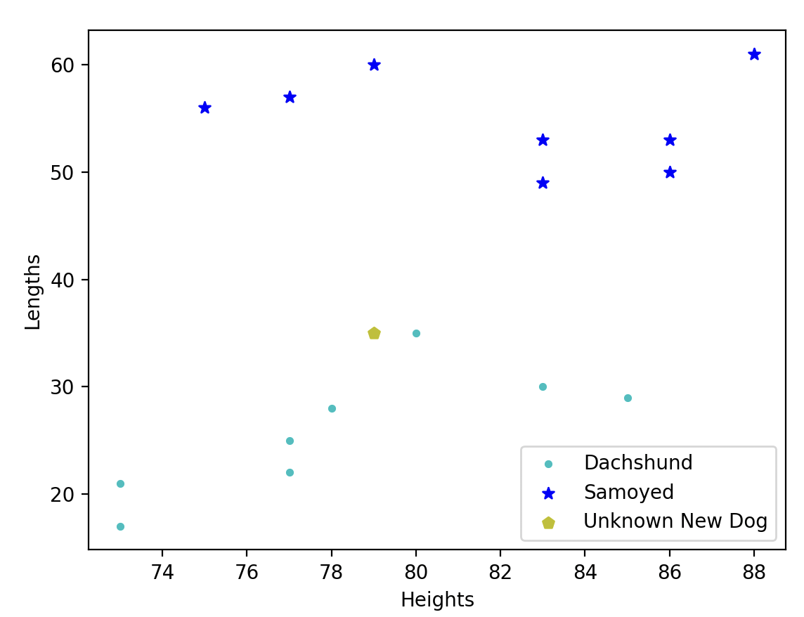 |
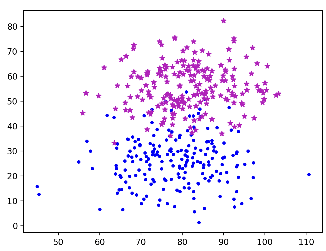 |
보면 원래의 데이터가 왼쪽이고, 데이터 증강을 통해 데이터셋을 늘린게 오른쪽과 같아요!
한 눈에 봐도 학습이 잘 되었다는걸 알 수 있지요! 😊
딥러닝으로 넘어가볼까요?
딥러닝 - MLP (Multi Layer Perception)
소개
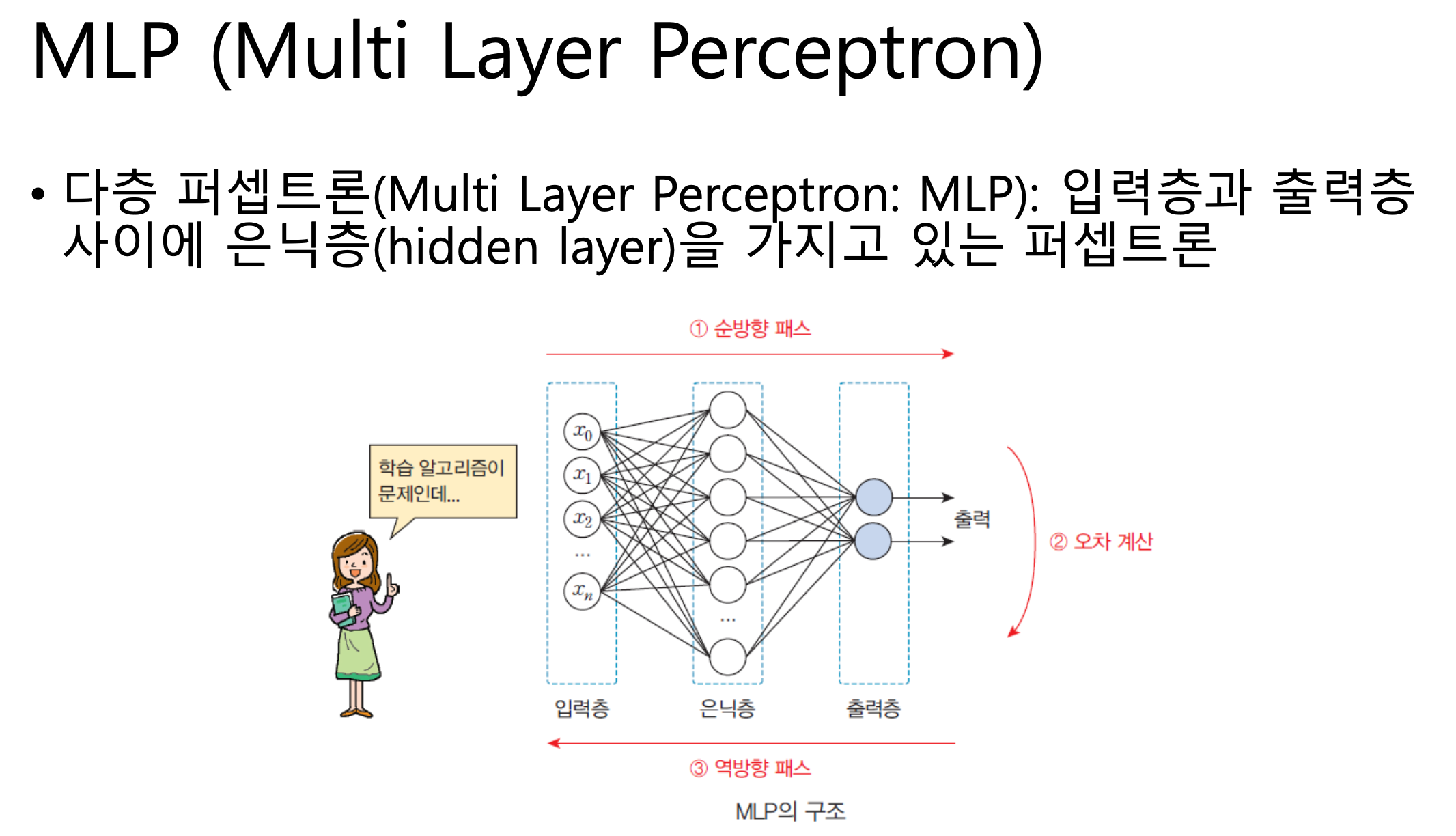
입력층은 신경망, 뉴런과 같은 역할을 해요
은닉층은 내가 원하는 형태로 구성해서 좀 더 깊은 구조의 학습이 가능해요
딥러닝에서는 입력데이터와 출력데이터의 크기가 매우매우 중요해요!
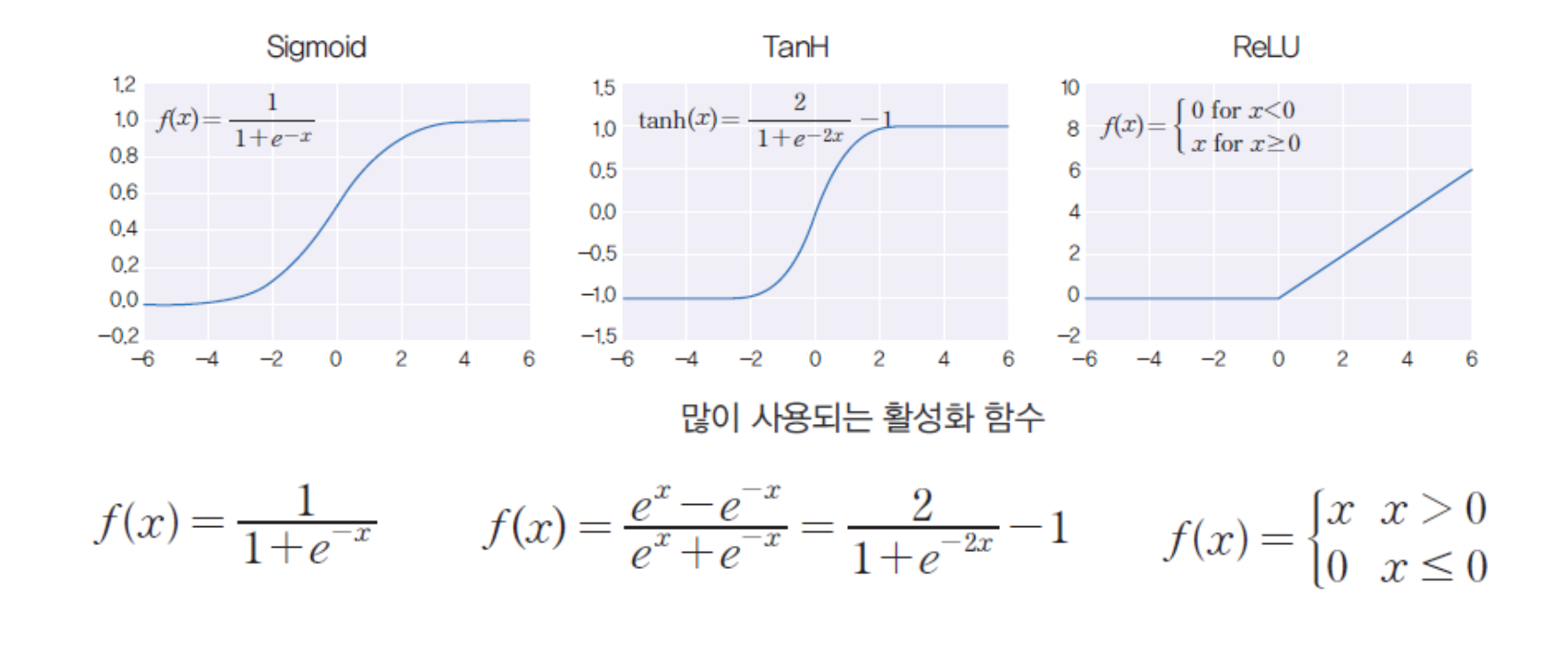
활성화 함수
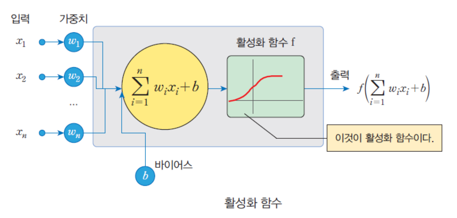
활성화 함수(activation function)는 입력의 총합을 받아서 출력
값을 계산하는 함수에요.
MLP에서는 다양한 활성화 함수를 사용하는데,
그 중에서 많이 쓰이는 세가지 함수를 소개할게요!
손실 함수
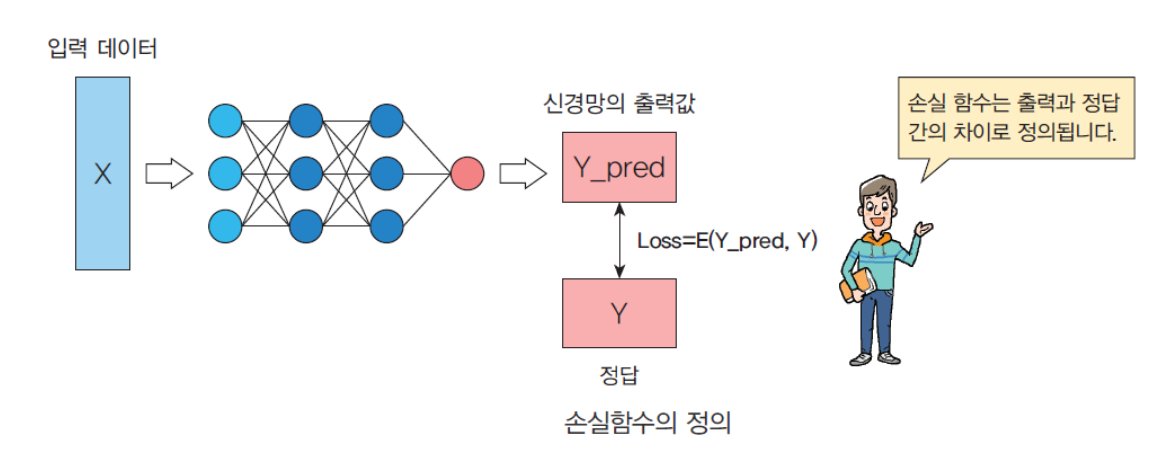
신경망에서 학습을 시킬 때는 실제 출력과 원하는 출력 사이의
오차를 이용해요.
이때 오차를 계산하는 함수를
손실함수(loss function)라고 해요.
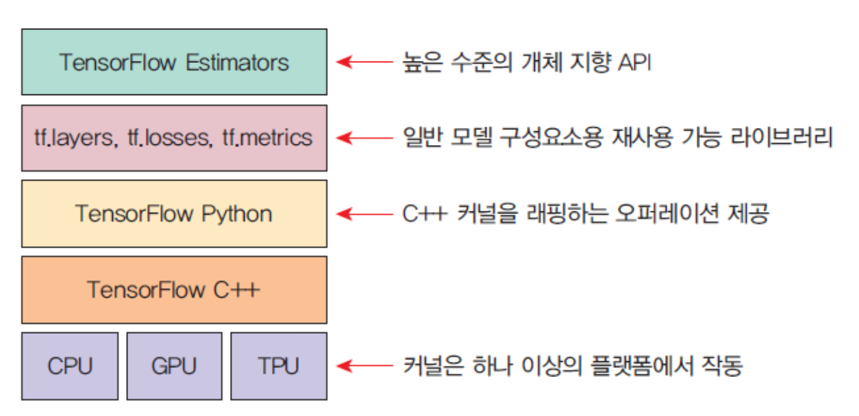
TensorFlow
텐서플로우(TensorFlow)는 딥러닝 프레임워크의 일종으로, 텐서
플로우는 내부적으로 C/C++로 구현되어 있고 파이썬을 비룻하
여 여러 가지 언어에서 접근할 수 있도록 인터페이스를 제공해줘요!
케라스는 파이썬으로 작성되었으며, 고수준 딥러닝 API입니다!
케라스에서는 여러 가지 백엔드를 선택할 수 있지만,
아무래도 가장 많이 선택되는 백엔드는 텐서플로우랍니다
케라스의 장점
쉽고 빠른 프로토타이핑이 가능하다.
피드포워드 신경망, 컨볼루션 신경망과 순환 신경망은 물론, 여러 가지의 조합도 지원한다.
CPU 및 GPU에서 원활하게 실행된다.
XOR을 학습하는 MLP
XOR이란?
Exclusive-OR
입력이 같으면 `0`, 다르면 `1`의 출력이 나오는 소자
- 입력 중 어느 하나만 1일 경우에만 출력이 1이 되는 소자 -
MLP로 XOR 게이트를 구현 해 볼게요!
import tensorflow as tf
model = tf.keras.models.Sequential()
model.add(tf.keras.layers.Dense(units=2, input_shape=(2,) ,activation="sigmoid",name="INPUT"))
model.add(tf.keras.layers.Dense(units=1, activation='sigmoid',name="OUTPUT"))
model.compile(loss="mse",optimizer=tf.keras.optimizers.SGD(0.3))
print(model.summary())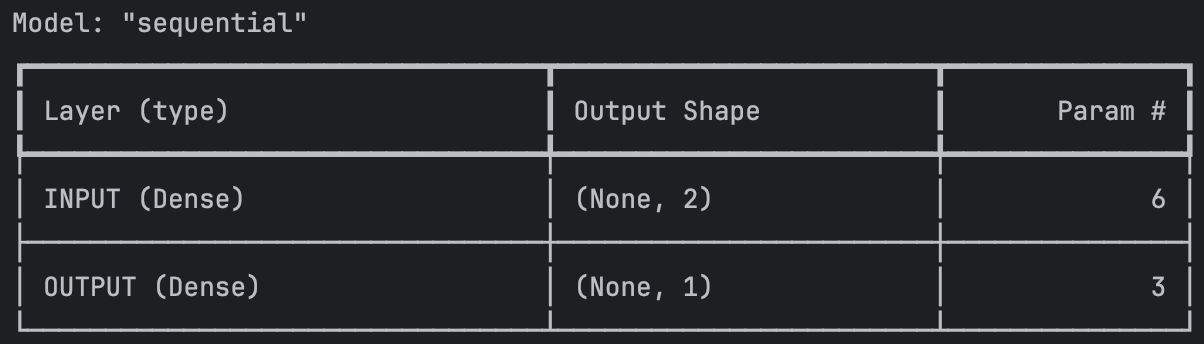
레이어가 2층으로 쌓인 SDG 모델을 만들어줄게요
X = tf.constant([[0,0],[0,1],[1,0],[1,1]])
y = tf.constant([0,1,1,0])
print(model.summary())
model.fit(X,y, batch_size=1, epochs=1000)
print(model.predict(X))
그리고 모델의 학습 데이터를 주고서
순서대로 0,1,1,0을 출력하도록 학습시켜줬어요
여러분이 직접 해볼때는 지금처럼 학습이 안될수도 있어요.
MLP 모델의 핵심은 epoch 와 SDG learning rate를 조절해가며 최적의 학습 모델을 찾는 것이랍니다!
화이트 노이즈 학습하기
혹시 노이즈 캔슬링의 원리를 알고 계시나요?
노이즈 캔슬링은 소리 파형의 반대 파형을 줘서 서로 상쇄시키는 기술이에요!
그러면 노이즈 캔슬링 기술의 첫번째 스텝은 소리의 파형을 계산하는 것 이겠지요
우리는 그 과정을 한 번 해볼게요 !
임의의 함수로 파형을 재현하고 그 파형을 학습시킬 수 있는지!
해보자구요~
필요 라이브러리 임포트
import numpy as np
import time
from matplotlib import pyplot as plt
from sklearn.model_selection import train_test_split
import tensorflow as tf
랜덤 값으로 함수 구현하기
SAMPLE_NUMBER = 10000
np.random.seed(int(time.time()))
Xs = np.random.uniform(low=-2.0, high=0.5,
                       size=SAMPLE_NUMBER)
np.random.shuffle(Xs)  # 랜덤 값에다가 한번 더 셔플
print(Xs[:10])
ys = (Xs + 1.7) * (Xs + 0.7) * (Xs - 0.2) * (Xs - 1.3) * (Xs - 1.9) + 0.2  # 5차 함수

ys += 0.1 * np.random.randn(SAMPLE_NUMBER)
np.save('noise.npy', ys)
Train-Test 데이터 나누기
(X_train, X_test, y_train, y_test) = train_test_split(Xs, ys, test_size=0.2)
print(X_train.shape, X_test.shape, y_train.shape, y_test.shape)

plt.plot(X_train, y_train, 'r.', label='Train')
plt.plot(X_test, y_test, 'b.', label='Test')

plt.legend()
plt.show()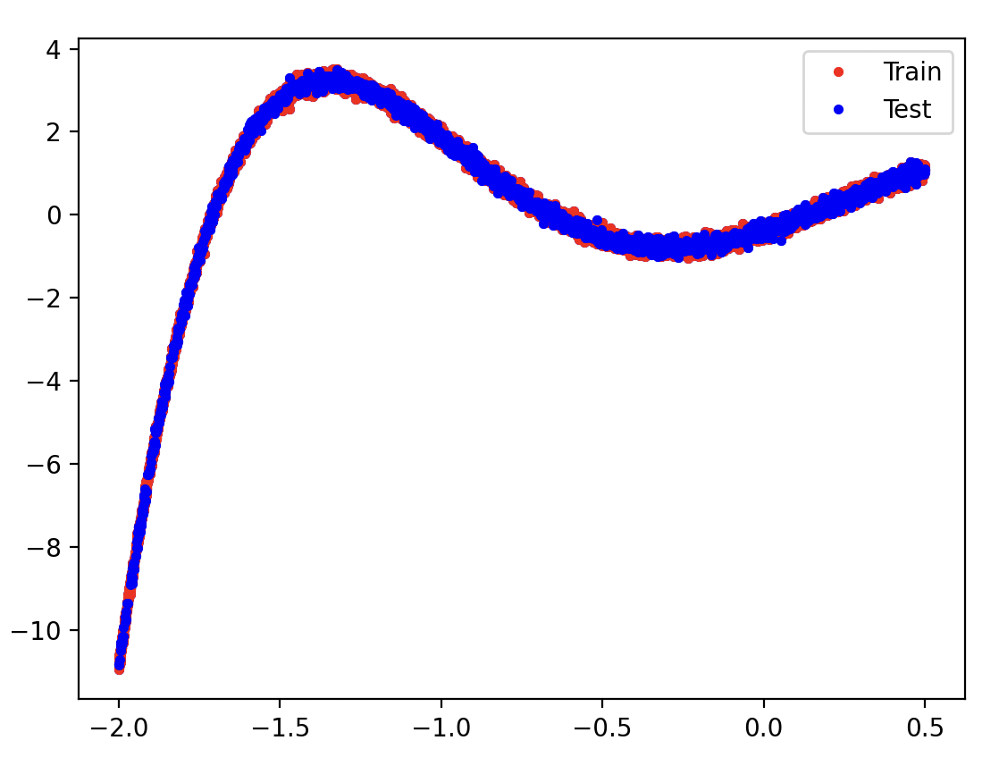
Train데이터와 Test데이터가 비슷한걸 보니 학습이 잘 됐나봐요 !
model = tf.keras.Sequential([], name='Model')
Input_layer = tf.keras.Input(shape=(1,))
model.add(Input_layer)
model.add(tf.keras.layers.Dense(
units=16, activation='relu', name="Layer1"))
model.add(tf.keras.layers.Dense(
units=16, activation='relu', name="Layer2"))
model.add(tf.keras.layers.Dense(
units=1, name="OUTPUT"))
model.summary()
model.compile(optimizer='adam', loss='mse')
history = model.fit(X_train, y_train, epochs=500)
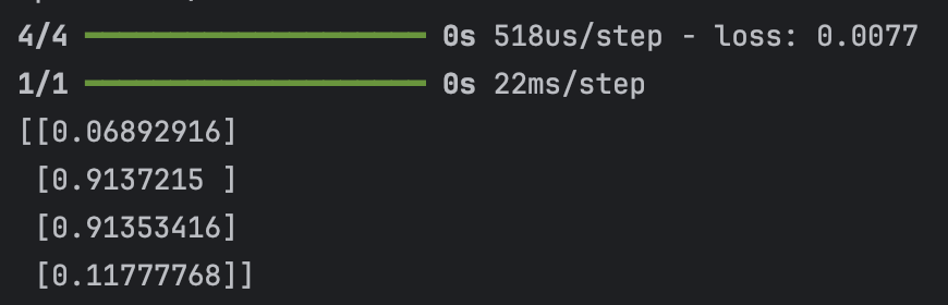
print(history.history['loss'])
y_pred = model.predict(X_test)
print(f'최종 정확도 : {model.evaluate(y_test, y_pred)}')
plt.plot(y_test, y_pred, 'r.')
plt.show()
plt.plot(history.history['loss'])
plt.show()
Layer를 여러층 깔아주는 MLP 모델을 정의하고서 예측치를 만들어줬어요
이제 테스트 데이터와 예측치가 어느정도 일치하는지 그래프로 그리는 것 까지 해줬어요
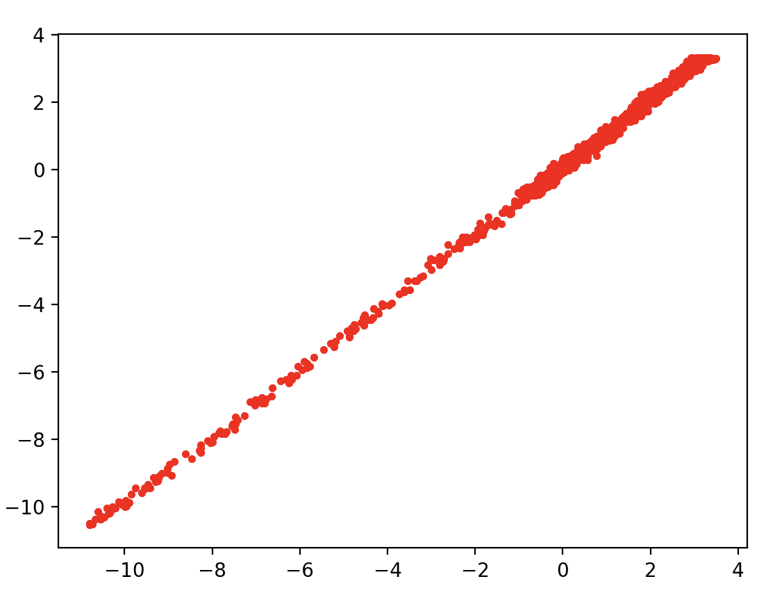
y=x 그래프를 그리는 걸 보니 예측치가 잘 들어맞았다는 걸 알 수 있어요!
오늘은 여기까지!
다음시간에도 유익한 정보로 찾아뵐게요~!

'ABC 부트캠프' 카테고리의 다른 글
| [23일차] ABC 부트캠프 - 신경망 모델 (CNN을 활용한 예제 학습) (0) | 2024.07.24 |
|---|---|
| [22일차] ABC 부트캠프 - MNIST 필기체 데이터 학습 (0) | 2024.07.23 |
| [20일차] ABC 부트캠프 - ESG 강연 #2 (2) | 2024.07.21 |
| [19일차] ABC 부트캠프 - 인공지능 기초 ( 데이터셋 학습) (1) | 2024.07.21 |
| [18일차] ABC 부트캠프 - 인공지능 기초 (PyCharm 설치 & 선형 회귀) (0) | 2024.07.17 |


